3.3 Hypothesis testing
3.3.1 t-Testing
3.3.1.1 Variance
3.3.1.2 t-Test
3.3.1.3 Implementation
Consider the following linear model for the wage: \[\text{wage}_i=\beta_0+\beta_1\text{educ}_i+\beta_2\text{exper}_i+\beta_3\text{tenure}_i+e_i\] That is, hourly wage is a linear function of education, work experience, and tenure (years with current employer). As we have already seen, basic hypothesis testing statistics are provided using the summary command on a linear model:
modela <- lm(wage~educ+exper+tenure,data=wage1)
summary(modela)
##
## Call:
## lm(formula = wage ~ educ + exper + tenure, data = wage1)
##
## Residuals:
## Min 1Q Median 3Q Max
## -7.6498 -1.7708 -0.6407 1.2051 14.7201
##
## Coefficients:
## Estimate Std. Error t value Pr(>|t|)
## (Intercept) -2.91354 0.73172 -3.982 7.81e-05 ***
## educ 0.60268 0.05148 11.708 < 2e-16 ***
## exper 0.02252 0.01210 1.861 0.0633 .
## tenure 0.17002 0.02173 7.825 2.83e-14 ***
## ---
## Signif. codes: 0 '***' 0.001 '**' 0.01 '*' 0.05 '.' 0.1 ' ' 1
##
## Residual standard error: 3.096 on 522 degrees of freedom
## Multiple R-squared: 0.3072, Adjusted R-squared: 0.3032
## F-statistic: 77.15 on 3 and 522 DF, p-value: < 2.2e-16This allows us to test hypotheses such as \(\beta_1=0\) or \(\beta_2=0\). In this case, the \(t\)-statistic for the null \(\mathcal{H}_0:\beta_1=0\) is \(11.708\) and the \(p\)-value for the test against the two-sided alternative is \(< 2\times10^{-16}\approx0\). Thus we can reject the null hypothesis even at even the \(0.1\%\) level. We have also seen that we can use the broom package to get testing statistics:
tidy(modela)## # A tibble: 4 x 5
## term estimate std.error statistic p.value
## <chr> <dbl> <dbl> <dbl> <dbl>
## 1 (Intercept) -2.91 0.732 -3.98 7.81e- 5
## 2 educ 0.603 0.0515 11.7 2.83e-28
## 3 exper 0.0225 0.0121 1.86 6.33e- 2
## 4 tenure 0.170 0.0217 7.83 2.83e-143.3.1.4 Testing complex hypotheses
Now suppose we want to test a more diffucult hypothesis such as: \[\mathcal{H}_0:\beta_2=\beta_3, \enspace\enspace\mathcal{H}_1:\beta_2\neq\beta_3\] While it is possible to get R to give us the answer to this test, it is usually much easier to do some algebra to manipulate the model into testing the hypothesis for us. Consider our null hypothesis. We are going to set this null equal to zero and “reparameterize” the model. First: \[\beta_2=\beta_3\] \[\beta_2-\beta_3=0\] \[\theta_0=0\] This means that \(\theta_0=\beta_2-\beta_3\). We need to transform our original model to use \(\theta_0\) instead of either \(\beta_2\) or \(\beta_3\). Since \(\theta_0+\beta_3=\beta_2\), we are going to substitute \(\theta_0+\beta_3\) for \(\beta_2\) in the original equation: \[\text{wage}_i=\beta_0+\beta_1\text{educ}_i+(\theta_0+\beta_3)\text{exper}_i+\beta_3\text{tenure}_i+e_i\] Distributing the experience term we see that: \[\text{wage}_i=\beta_0+\beta_1\text{educ}_i+(\theta_0\text{exper}_i+\beta_3\text{exper}_i)+\beta_3\text{tenure}_i+e_i\] Combining like terms we find \[\text{wage}_i=\beta_0+\beta_1\text{educ}_i+\theta_0\text{exper}_i+(\beta_3\text{exper}_i+\beta_3\text{tenure}_i)+e_i\] or \[\text{wage}_i=\beta_0+\beta_1\text{educ}_i+\theta_0\text{exper}_i+\beta_3(\text{exper}_i+\text{tenure}_i)+e_i\] Now we are going to run this model:
modelb <- lm(wage~educ+exper+I(exper+tenure),data=wage1)
summary(modelb)
##
## Call:
## lm(formula = wage ~ educ + exper + I(exper + tenure), data = wage1)
##
## Residuals:
## Min 1Q Median 3Q Max
## -7.6498 -1.7708 -0.6407 1.2051 14.7201
##
## Coefficients:
## Estimate Std. Error t value Pr(>|t|)
## (Intercept) -2.91354 0.73172 -3.982 7.81e-05 ***
## educ 0.60268 0.05148 11.708 < 2e-16 ***
## exper -0.14749 0.02975 -4.958 9.63e-07 ***
## I(exper + tenure) 0.17002 0.02173 7.825 2.83e-14 ***
## ---
## Signif. codes: 0 '***' 0.001 '**' 0.01 '*' 0.05 '.' 0.1 ' ' 1
##
## Residual standard error: 3.096 on 522 degrees of freedom
## Multiple R-squared: 0.3072, Adjusted R-squared: 0.3032
## F-statistic: 77.15 on 3 and 522 DF, p-value: < 2.2e-16modelb has exactly the same \(R^2\) value as modela because they are exactly the same line through the data. We have only transformed the units we are using to measure the variables. You will notice that \(\beta_0\) and \(\beta_1\) are exactly the same between these two models. You will also see that even though we transformed the third variable, \(\beta_3\) is the same in both models. The only difference is that where \(\beta_2\) should be, we now have \(\theta_0\) or the difference between \(\beta_2\) and \(\beta_3\). Because this value is now one of our coefficients, we can test the hypothesis by looking at the \(t\)-statistic (\(-4.958\)) and \(p\)-value (\(\approx0\)). We find that we can reject the null hypothesis at even the \(0.1\%\) level.
3.3.1.5 Confidence intervals
We can obtain confidence intervals for the \(\beta\)s by calling:
confint(modela)## 2.5 % 97.5 %
## (Intercept) -4.351015282 -1.47606888
## educ 0.501556068 0.70381214
## exper -0.001250762 0.04629998
## tenure 0.127336330 0.21270003We can also use the broom package:
tidy(modela,conf.int=TRUE)## # A tibble: 4 x 7
## term estimate std.error statistic p.value conf.low conf.high
## <chr> <dbl> <dbl> <dbl> <dbl> <dbl> <dbl>
## 1 (Intercept) -2.91 0.732 -3.98 7.81e- 5 -4.35 -1.48
## 2 educ 0.603 0.0515 11.7 2.83e-28 0.502 0.704
## 3 exper 0.0225 0.0121 1.86 6.33e- 2 -0.00125 0.0463
## 4 tenure 0.170 0.0217 7.83 2.83e-14 0.127 0.213If we want confidence intervals for a prediction, it is possible to modify our model to get the result that we want. Suppose we want to make a predict for a person with \(16\) years of education, \(5\) years of experience, and \(1\) year of tenure. For this person, we want to predict: \[\theta_1=\beta_0+20\beta_1+5\beta_2+\beta_3\] or \[\beta_0=\theta_1-20\beta_1-5\beta_2-\beta_3\] Substituting we find \[\text{wage}_i=(\theta_1-20\beta_1-5\beta_2-\beta_3)+\beta_1\text{educ}_i+\beta_2\text{exper}_i+\beta_3\text{tenure}_i+e_i\] or \[\text{wage}_i=\theta_1+\beta_1(\text{educ}_i-20)+\beta_2(\text{exper}_i-5)+\beta_3(\text{tenure}_i-1)+e_i\] So if we run the following:
confint(lm(wage~I(educ-20)+I(exper-5)+I(tenure-1),data=wage1))## 2.5 % 97.5 %
## (Intercept) 8.653028322 10.19253410
## I(educ - 20) 0.501556068 0.70381214
## I(exper - 5) -0.001250762 0.04629998
## I(tenure - 1) 0.127336330 0.21270003We find that the predicted wage will be between \(\$8.65/hr\) and \(\$10.19/hr\) with \(95\%\) confidence.
3.3.2 Anova
3.3.3 Heteroskedasticity
dt$x <- rnorm(bigN,2,1)
dt$y <- 2*dt$x + rnorm(bigN,0,abs(dt$x-2))
result <- dt[,tidy(lm(y~x))[2,],by=.(n,sim)]view.sim(result)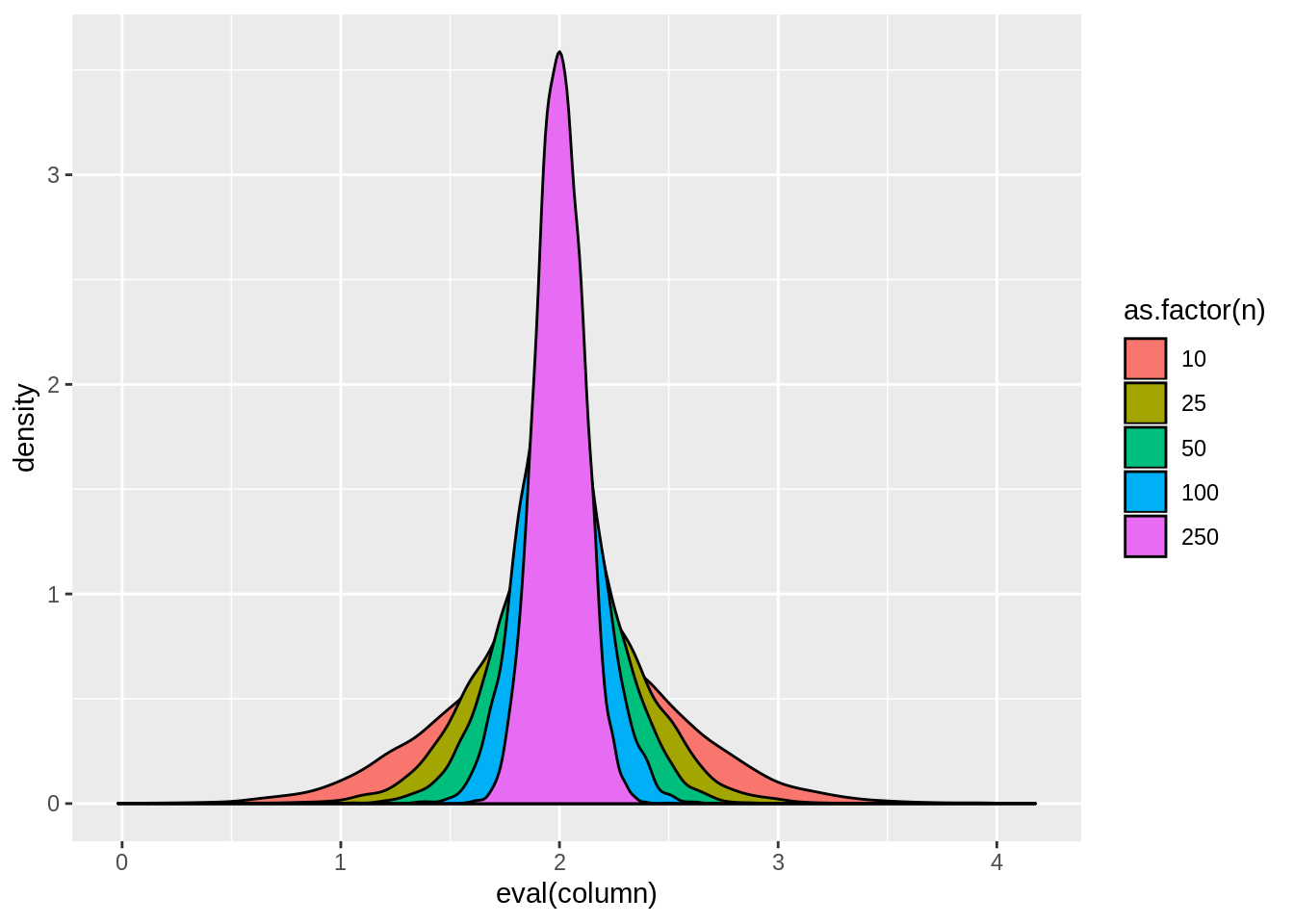
view.sim(result,quote(tstat1))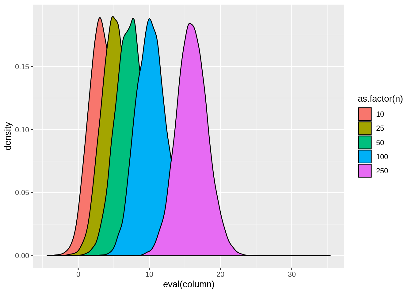
view.sim(result,quote(tstat2))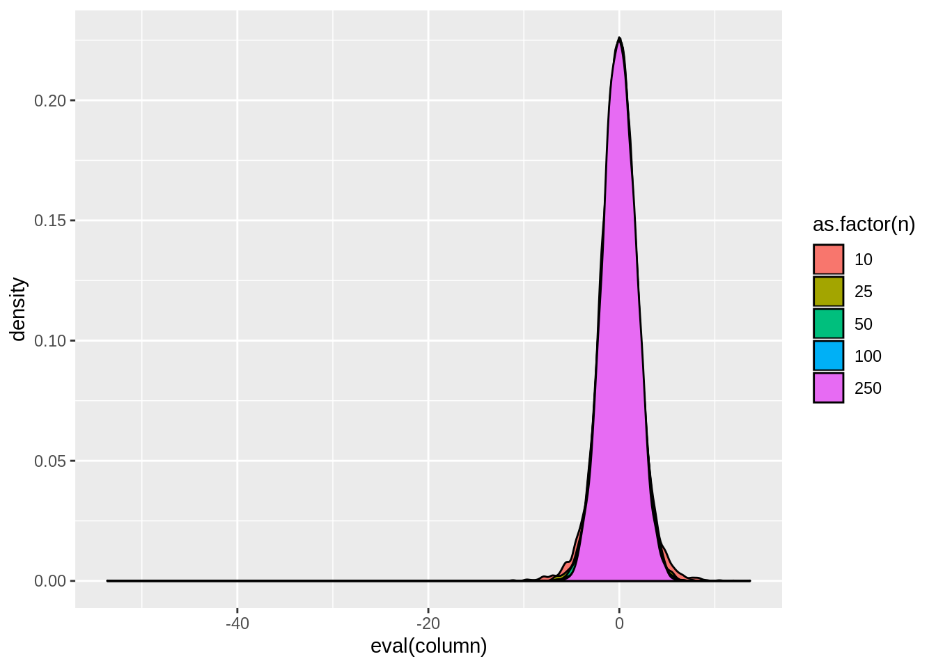
result[,lapply(.SD,mean),by=n]## n sim estimate std.error statistic p.value tstat1
## 1: 10 5000.5 2.002368 0.28925600 8.064719 3.906233e-03 4.030707
## 2: 25 15000.5 1.999819 0.19145331 11.042417 5.710813e-05 5.516472
## 3: 50 25000.5 2.000062 0.13822892 14.880942 4.821769e-09 7.441809
## 4: 100 35000.5 2.000140 0.09876214 20.547341 4.984584e-21 10.274640
## 5: 250 45000.5 2.000436 0.06295988 31.962402 1.201828e-57 15.986087
## tstat2 reject1 reject2
## 1: -0.003305041 0.8011 0.2875
## 2: -0.009472007 0.9617 0.2750
## 3: 0.002675460 0.9965 0.2686
## 4: 0.001938765 0.9999 0.2647
## 5: 0.009772447 1.0000 0.26193.3.4 White correction
To implement the white correction, we can use the following packages:
library(lmtest)
library(sandwich)
It is possible to use only sandwich by modifying the tidy function to allow for different variance-covariances of \(\hat\beta\). This is a good exercise and is left for the reader. To use the lmtest functions instead simply type:
coeftest(modela,sandwich::vcovHC)##
## t test of coefficients:
##
## Estimate Std. Error t value Pr(>|t|)
## (Intercept) -2.913542 0.824687 -3.5329 0.0004475 ***
## educ 0.602684 0.062351 9.6660 < 2.2e-16 ***
## exper 0.022525 0.010697 2.1057 0.0357096 *
## tenure 0.170018 0.029907 5.6850 2.179e-08 ***
## ---
## Signif. codes: 0 '***' 0.001 '**' 0.01 '*' 0.05 '.' 0.1 ' ' 1for hypothesis testing or
coefci(modela,vcov=sandwich::vcovHC)## 2.5 % 97.5 %
## (Intercept) -4.533655572 -1.29342859
## educ 0.480194101 0.72517411
## exper 0.001509962 0.04353926
## tenure 0.111266198 0.22877016for confidence intervals.
result <- dt[,tidyw(lm(y~x))[2,],by=.(n,sim)]view.sim(result)
view.sim(result,quote(tstat1))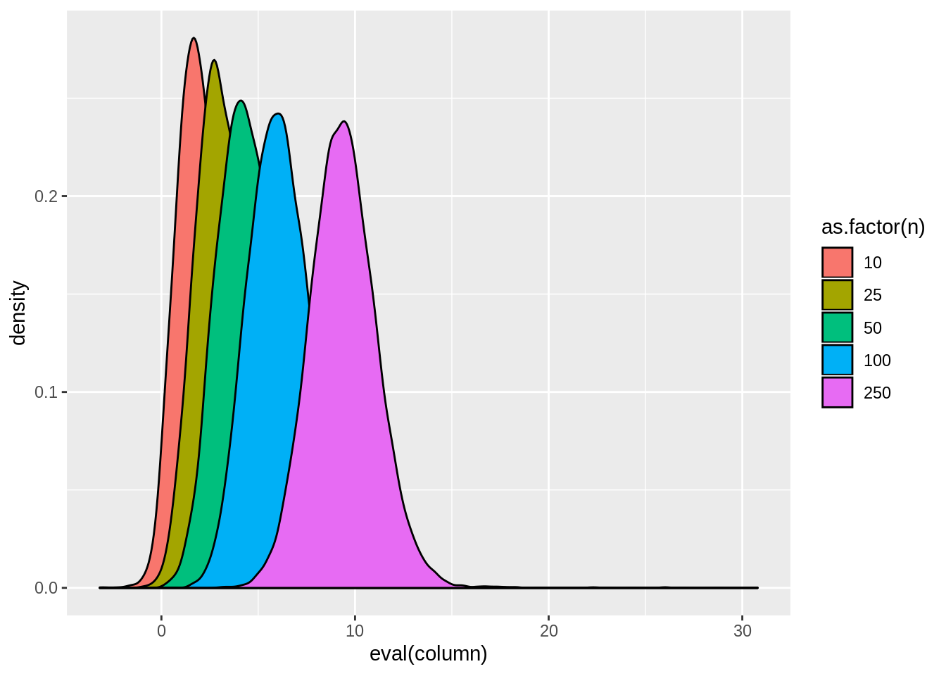
view.sim(result,quote(tstat2))
result[,lapply(.SD,mean),by=n]## n sim estimate std.error statistic p.value tstat1
## 1: 10 5000.5 2.002368 0.5083918 5.377784 2.007332e-02 2.691747
## 2: 25 15000.5 1.999819 0.3319309 6.952406 1.580453e-03 3.471984
## 3: 50 25000.5 2.000062 0.2387368 9.094348 7.709852e-05 4.548308
## 4: 100 35000.5 2.000140 0.1703459 12.295774 4.114901e-08 6.149056
## 5: 250 45000.5 2.000436 0.1088193 18.785425 8.372739e-16 9.396102
## tstat2 reject1 reject2
## 1: 0.005709102 0.5594 0.1195
## 2: -0.008438554 0.8220 0.0846
## 3: 0.002267485 0.9626 0.0717
## 4: 0.002337081 0.9984 0.0625
## 5: 0.006778376 1.0000 0.05493.3.5 White test
3.3.6 General least squares
3.3.7 Weighted least squares
To implement weighted least squares, first we need to take a model and get its residuals. To do this, we are going to use the augment function from the broom package, but it is just as easy to do with residuals function in base R:
dt <- augment(modela)
dt$ynew <- log(dt$.resid^2)
Notice, we squared the residuals and took the natural logarithm because we are interested in modeling the variance of the residuals which is the squared deviation from the mean (\(0\) for residuals). Now we are going to model the residual variance in a new model:
modelc <- lm(ynew~educ+exper+tenure,data=dt)Using this new model, we can estimate (or forecast/predict) the residual variance:
dt <- augment(modelc)
wage1$h <- exp(dt$.fitted)
These are the weights we are going to use in our weighted least squares. Now we can run WLS using the weights option in the lm command:
modeld <- lm(wage~educ+exper+tenure,weights=1/h,data=wage1)
summary(modeld)
##
## Call:
## lm(formula = wage ~ educ + exper + tenure, data = wage1, weights = 1/h)
##
## Weighted Residuals:
## Min 1Q Median 3Q Max
## -4.4935 -1.3978 -0.4832 0.9871 12.3336
##
## Coefficients:
## Estimate Std. Error t value Pr(>|t|)
## (Intercept) 0.592993 0.417042 1.422 0.155652
## educ 0.298097 0.031815 9.370 < 2e-16 ***
## exper 0.031655 0.009327 3.394 0.000742 ***
## tenure 0.150488 0.024438 6.158 1.47e-09 ***
## ---
## Signif. codes: 0 '***' 0.001 '**' 0.01 '*' 0.05 '.' 0.1 ' ' 1
##
## Residual standard error: 2.135 on 522 degrees of freedom
## Multiple R-squared: 0.2094, Adjusted R-squared: 0.2049
## F-statistic: 46.09 on 3 and 522 DF, p-value: < 2.2e-16