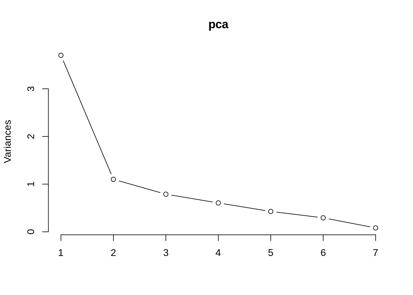
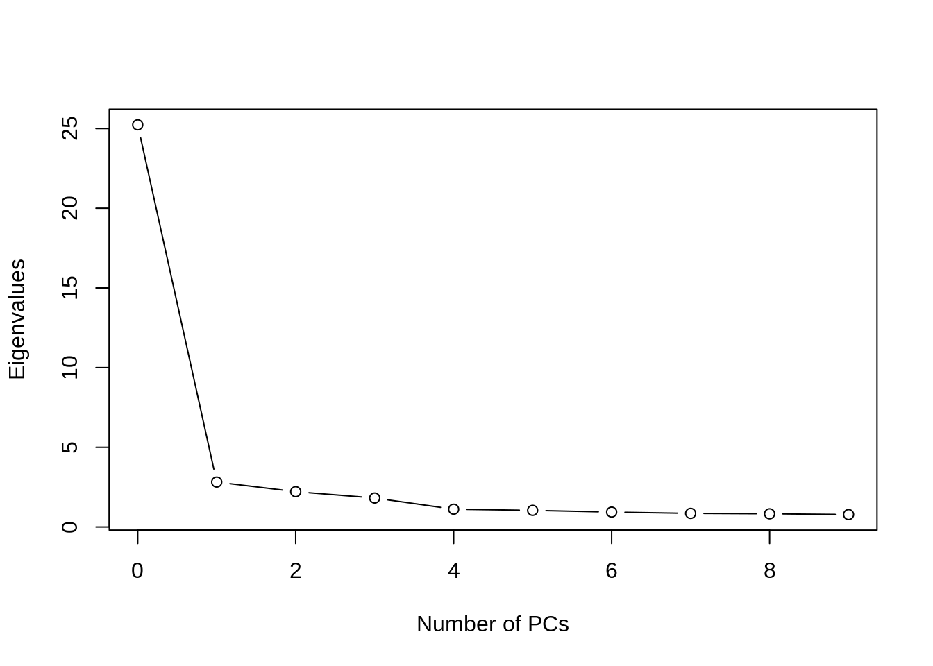
Common factor models
hprice2$fact <- scale(pca$x[,1])
var(hprice2$fact)
## [1] 1
# modeling with the factors
model0 <- lm(log(price)~log(nox),data=hprice2)
summary(model0)
##
## Call:
## lm(formula = log(price) ~ log(nox), data = hprice2)
##
## Residuals:
##      Min       1Q   Median       3Q      Max
## -1.17062 -0.19368 -0.02582  0.18385  1.09366
##
## Coefficients:
##             Estimate Std. Error t value Pr(>|t|)
## (Intercept) 11.70719    0.13243   88.40   <2e-16 ***
## log(nox)    -1.04314    0.07767  -13.43   <2e-16 ***
## ---
## Signif. codes:  0 '***' 0.001 '**' 0.01 '*' 0.05 '.' 0.1 ' ' 1
##
## Residual standard error: 0.3516 on 504 degrees of freedom
## Multiple R-squared:  0.2636, Adjusted R-squared:  0.2621
## F-statistic: 180.4 on 1 and 504 DF,  p-value: < 2.2e-16
model1 <- lm(log(price)~fact,data=hprice2)
summary(model1)
##
## Call:
## lm(formula = log(price) ~ fact, data = hprice2)
##
## Residuals:
##      Min       1Q   Median       3Q      Max
## -0.78445 -0.16469 -0.03504  0.14551  1.24032
##
## Coefficients:
##             Estimate Std. Error t value Pr(>|t|)
## (Intercept)  9.94106    0.01219  815.47   <2e-16 ***
## fact        -0.30404    0.01220  -24.92   <2e-16 ***
## ---
## Signif. codes:  0 '***' 0.001 '**' 0.01 '*' 0.05 '.' 0.1 ' ' 1
##
## Residual standard error: 0.2742 on 504 degrees of freedom
## Multiple R-squared:  0.5519, Adjusted R-squared:  0.551
## F-statistic: 620.8 on 1 and 504 DF,  p-value: < 2.2e-16
model2 <- lm(log(price)~log(nox)+fact,data=hprice2)
summary(model2)
##
## Call:
## lm(formula = log(price) ~ log(nox) + fact, data = hprice2)
##
## Residuals:
##      Min       1Q   Median       3Q      Max
## -0.77893 -0.16266 -0.03565  0.14315  1.23570
##
## Coefficients:
##             Estimate Std. Error t value Pr(>|t|)
## (Intercept)  9.67179    0.15239  63.468   <2e-16 ***
## log(nox)     0.15904    0.08972   1.773   0.0769 .
## fact        -0.32771    0.01807 -18.135   <2e-16 ***
## ---
## Signif. codes:  0 '***' 0.001 '**' 0.01 '*' 0.05 '.' 0.1 ' ' 1
##
## Residual standard error: 0.2736 on 503 degrees of freedom
## Multiple R-squared:  0.5547, Adjusted R-squared:  0.5529
## F-statistic: 313.3 on 2 and 503 DF,  p-value: < 2.2e-16
c(AIC(model0),AIC(model1),AIC(model2))
## [1] 382.0341 130.6135 129.4623
c(BIC(model0),BIC(model1),BIC(model2))
## [1] 394.7137 143.2931 146.3684
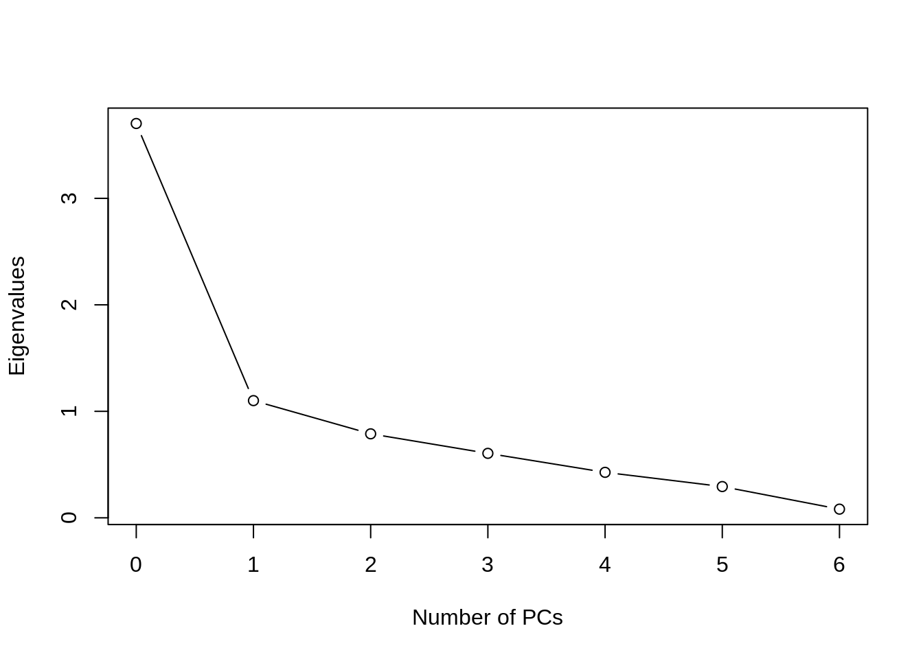
Time series factor models
french <- fread('french.csv')
french$Date <- as.Date(french$Date)
panel <- french[,2:50]
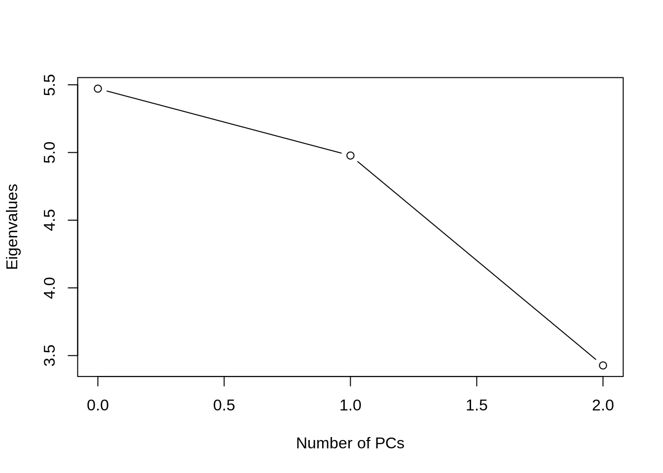
pca <- prcomp(panel,scale=TRUE)
pca.select(pca)
## [1] 1 1
french$factor <- pca$x[,1]
french$factor <- scale(french$factor)
colnames(french)
##  [1] "Date"   "Agric"  "Food"   "Soda"   "Beer"   "Smoke"  "Toys"
##  [8] "Fun"    "Books"  "Hshld"  "Clths"  "Hlth"   "MedEq"  "Drugs"
## [15] "Chems"  "Rubbr"  "Txtls"  "BldMt"  "Cnstr"  "Steel"  "FabPr"
## [22] "Mach"   "ElcEq"  "Autos"  "Aero"   "Ships"  "Guns"   "Gold"
## [29] "Mines"  "Coal"   "Oil"    "Util"   "Telcm"  "PerSv"  "BusSv"
## [36] "Hardw"  "Softw"  "Chips"  "LabEq"  "Paper"  "Boxes"  "Trans"
## [43] "Whlsl"  "Rtail"  "Meals"  "Banks"  "Insur"  "RlEst"  "Fin"
## [50] "Other"  "factor"
##      Agric       Food       Soda       Beer      Smoke       Toys
## 0.12021240 0.13155467 0.11531338 0.12442778 0.09174715 0.14971971
##        Fun      Books      Hshld      Clths       Hlth      MedEq
## 0.15280831 0.16031235 0.14662061 0.15301802 0.13344679 0.14256020
##      Drugs      Chems      Rubbr      Txtls      BldMt      Cnstr
## 0.12516812 0.16174124 0.16094593 0.14574188 0.16838879 0.15685418
##      Steel      FabPr       Mach      ElcEq      Autos       Aero
## 0.14548138 0.13559541 0.16614923 0.16256363 0.14603539 0.15356122
##      Ships       Guns       Gold      Mines       Coal        Oil
## 0.13608411 0.11944298 0.04928365 0.12869771 0.09540056 0.11383108
##       Util      Telcm      PerSv      BusSv      Hardw      Softw
## 0.10618328 0.12927581 0.14744673 0.17239912 0.12876272 0.12809929
##      Chips      LabEq      Paper      Boxes      Trans      Whlsl
## 0.14723511 0.15488890 0.15675136 0.14541913 0.16181750 0.16966150
##      Rtail      Meals      Banks      Insur      RlEst        Fin
## 0.15603055 0.15567743 0.15014514 0.15235295 0.14690598 0.16029714
##      Other
## 0.14788972
modely <- lm(Fin~factor,data=french)
summary(modely)
##
## Call:
## lm(formula = Fin ~ factor, data = french)
##
## Residuals:
##      Min       1Q   Median       3Q      Max
## -13.7553  -1.6724   0.0878   1.7345  15.0728
##
## Coefficients:
##             Estimate Std. Error t value Pr(>|t|)
## (Intercept)   1.1078     0.1328   8.341 5.25e-16 ***
## factor        5.3737     0.1329  40.425  < 2e-16 ***
## ---
## Signif. codes:  0 '***' 0.001 '**' 0.01 '*' 0.05 '.' 0.1 ' ' 1
##
## Residual standard error: 3.226 on 588 degrees of freedom
## Multiple R-squared:  0.7354, Adjusted R-squared:  0.7349
## F-statistic:  1634 on 1 and 588 DF,  p-value: < 2.2e-16
modelx <- lm(Gold~factor,data=french)
summary(modelx)
##
## Call:
## lm(formula = Gold ~ factor, data = french)
##
## Residuals:
##     Min      1Q  Median      3Q     Max
## -28.629  -6.427  -0.743   5.707  76.339
##
## Coefficients:
##             Estimate Std. Error t value Pr(>|t|)
## (Intercept)   0.8529     0.4317   1.975   0.0487 *
## factor        2.8640     0.4321   6.628 7.72e-11 ***
## ---
## Signif. codes:  0 '***' 0.001 '**' 0.01 '*' 0.05 '.' 0.1 ' ' 1
##
## Residual standard error: 10.49 on 588 degrees of freedom
## Multiple R-squared:  0.06951,    Adjusted R-squared:  0.06793
## F-statistic: 43.93 on 1 and 588 DF,  p-value: 7.715e-11
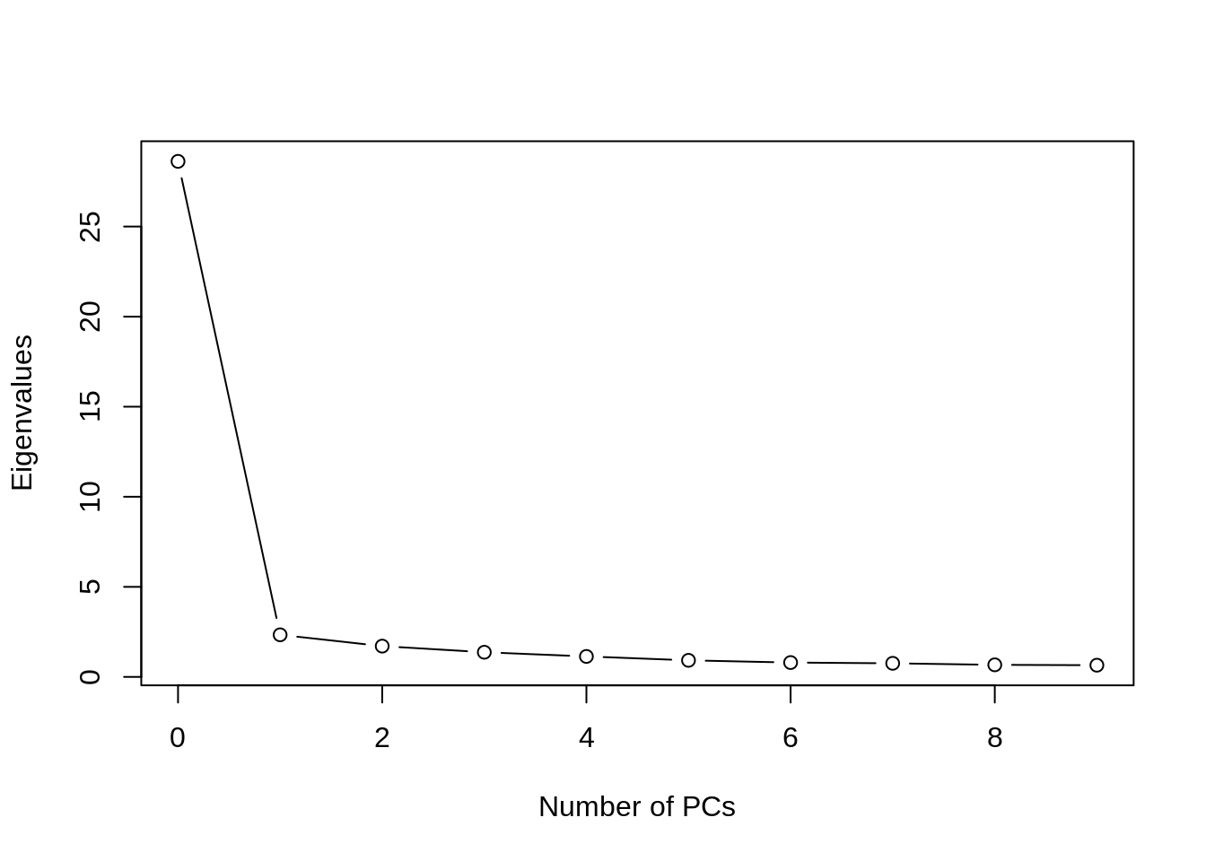
Testing common factors
french <- fread('french.csv')
market <- fread('market.csv')
french <- merge(french,market,all=FALSE)
french$Mkt <- as.numeric(french$Mkt)
## Warning: NAs introduced by coercion
french$SMB <- as.numeric(french$SMB)
## Warning: NAs introduced by coercion
french$HML <- as.numeric(french$HML)
## Warning: NAs introduced by coercion
french$Date <- as.Date(french$Date)
french <- french[complete.cases(french)]
panel <- french[,2:50]
french$factor <- scale(prcomp(panel,scale=TRUE)$x[,1])
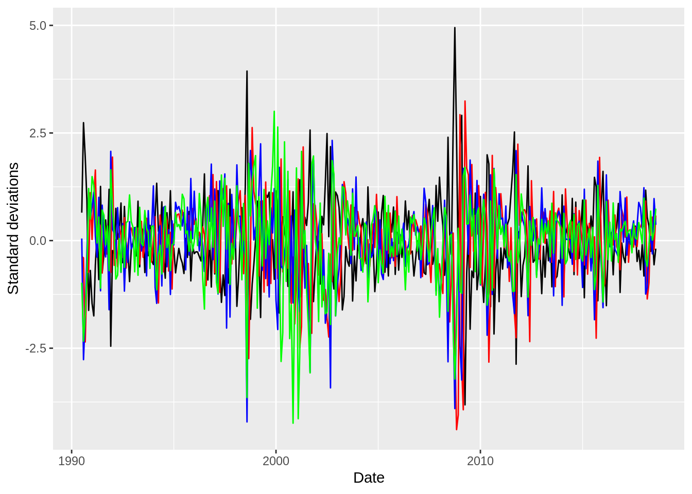
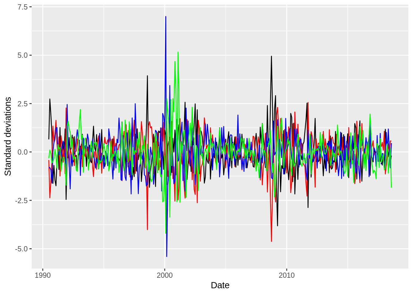
ggplot(french,aes(x=Date)) +
geom_line(aes(y=scale(factor)),color="black") +
geom_line(aes(y=scale(sp500)),color="red") +
geom_line(aes(y=scale(djia)),color="blue") +
geom_line(aes(y=scale(nasdaq)),color="green") +
scale_y_continuous('Standard deviations')
ggplot(french,aes(x=Date)) +
  geom_line(aes(y=scale(factor)),color="black") +
  geom_line(aes(y=scale(Mkt)),color="red") +
  geom_line(aes(y=scale(SMB)),color="blue") +
  geom_line(aes(y=scale(HML)),color="green") +
  scale_y_continuous('Standard deviations')
summary(lm(Fin~factor,data=french))
##
## Call:
## lm(formula = Fin ~ factor, data = french)
##
## Residuals:
##      Min       1Q   Median       3Q      Max
## -13.0272  -2.2469   0.0608   2.1385  15.1774
##
## Coefficients:
##             Estimate Std. Error t value Pr(>|t|)
## (Intercept)   1.2347     0.2014   6.131 2.45e-09 ***
## factor       -5.6832     0.2017 -28.180  < 2e-16 ***
## ---
## Signif. codes:  0 '***' 0.001 '**' 0.01 '*' 0.05 '.' 0.1 ' ' 1
##
## Residual standard error: 3.702 on 336 degrees of freedom
## Multiple R-squared:  0.7027, Adjusted R-squared:  0.7018
## F-statistic: 794.1 on 1 and 336 DF,  p-value: < 2.2e-16
summary(lm(Fin~sp500,data=french))
##
## Call:
## lm(formula = Fin ~ sp500, data = french)
##
## Residuals:
##      Min       1Q   Median       3Q      Max
## -26.3147  -4.2093   0.3922   4.0427  22.0414
##
## Coefficients:
##             Estimate Std. Error t value Pr(>|t|)
## (Intercept)  1.10241    0.36931   2.985  0.00304 **
## sp500        0.21836    0.08478   2.575  0.01044 *
## ---
## Signif. codes:  0 '***' 0.001 '**' 0.01 '*' 0.05 '.' 0.1 ' ' 1
##
## Residual standard error: 6.724 on 336 degrees of freedom
## Multiple R-squared:  0.01936,    Adjusted R-squared:  0.01644
## F-statistic: 6.633 on 1 and 336 DF,  p-value: 0.01044
summary(lm(Fin~djia,data=french))
##
## Call:
## lm(formula = Fin ~ djia, data = french)
##
## Residuals:
##      Min       1Q   Median       3Q      Max
## -14.1732  -2.6053   0.0351   2.2839  16.6701
##
## Coefficients:
##             Estimate Std. Error t value Pr(>|t|)
## (Intercept)  0.36483    0.22505   1.621    0.106
## djia         1.33718    0.05494  24.337   <2e-16 ***
## ---
## Signif. codes:  0 '***' 0.001 '**' 0.01 '*' 0.05 '.' 0.1 ' ' 1
##
## Residual standard error: 4.085 on 336 degrees of freedom
## Multiple R-squared:  0.638,  Adjusted R-squared:  0.637
## F-statistic: 592.3 on 1 and 336 DF,  p-value: < 2.2e-16
summary(lm(Fin~nasdaq,data=french))
##
## Call:
## lm(formula = Fin ~ nasdaq, data = french)
##
## Residuals:
##      Min       1Q   Median       3Q      Max
## -19.4251  -2.2702   0.0978   2.0964  20.9242
##
## Coefficients:
##             Estimate Std. Error t value Pr(>|t|)
## (Intercept)  0.51370    0.22626    2.27   0.0238 *
## nasdaq       0.85070    0.03547   23.98   <2e-16 ***
## ---
## Signif. codes:  0 '***' 0.001 '**' 0.01 '*' 0.05 '.' 0.1 ' ' 1
##
## Residual standard error: 4.123 on 336 degrees of freedom
## Multiple R-squared:  0.6313, Adjusted R-squared:  0.6302
## F-statistic: 575.3 on 1 and 336 DF,  p-value: < 2.2e-16
summary(lm(Fin~djia+nasdaq,data=french))
##
## Call:
## lm(formula = Fin ~ djia + nasdaq, data = french)
##
## Residuals:
##      Min       1Q   Median       3Q      Max
## -17.8625  -2.2066  -0.3436   1.9587  16.5220
##
## Coefficients:
##             Estimate Std. Error t value Pr(>|t|)
## (Intercept)  0.31291    0.19306   1.621    0.106
## djia         0.78479    0.06874  11.417   <2e-16 ***
## nasdaq       0.48525    0.04397  11.037   <2e-16 ***
## ---
## Signif. codes:  0 '***' 0.001 '**' 0.01 '*' 0.05 '.' 0.1 ' ' 1
##
## Residual standard error: 3.503 on 335 degrees of freedom
## Multiple R-squared:  0.7346, Adjusted R-squared:  0.733
## F-statistic: 463.5 on 2 and 335 DF,  p-value: < 2.2e-16
summary(lm(Fin~Mkt+SMB+HML,data=french))
##
## Call:
## lm(formula = Fin ~ Mkt + SMB + HML, data = french)
##
## Residuals:
##      Min       1Q   Median       3Q      Max
## -17.3274  -1.8534  -0.0451   1.8337  12.3187
##
## Coefficients:
##             Estimate Std. Error t value Pr(>|t|)
## (Intercept) -0.08446    0.18004  -0.469  0.63928
## Mkt          1.42157    0.04403  32.289  < 2e-16 ***
## SMB          0.17703    0.06277   2.820  0.00508 **
## HML          0.13878    0.05824   2.383  0.01773 *
## ---
## Signif. codes:  0 '***' 0.001 '**' 0.01 '*' 0.05 '.' 0.1 ' ' 1
##
## Residual standard error: 3.22 on 334 degrees of freedom
## Multiple R-squared:  0.7765, Adjusted R-squared:  0.7745
## F-statistic: 386.8 on 3 and 334 DF,  p-value: < 2.2e-16
pc.test(panel,french$factor)

## [1] 0 0
pc.test(panel,french$djia)

## [1] 1 1
pc.test(panel,french[,.(djia,sp500,nasdaq)])

## [1] 1 1
pc.test(panel,french[,.(Mkt,HML)])
## [1] 0 0
summary(lm(factor~Mkt+HML,data=french))
##
## Call:
## lm(formula = factor ~ Mkt + HML, data = french)
##
## Residuals:
##     Min      1Q  Median      3Q     Max
## -1.2884 -0.1527 -0.0076  0.1525  0.7906
##
## Coefficients:
##              Estimate Std. Error t value Pr(>|t|)
## (Intercept)  0.223657   0.013745   16.27   <2e-16 ***
## Mkt         -0.238852   0.003303  -72.31   <2e-16 ***
## HML         -0.055054   0.004277  -12.87   <2e-16 ***
## ---
## Signif. codes:  0 '***' 0.001 '**' 0.01 '*' 0.05 '.' 0.1 ' ' 1
##
## Residual standard error: 0.2458 on 335 degrees of freedom
## Multiple R-squared:  0.9399, Adjusted R-squared:  0.9396
## F-statistic:  2622 on 2 and 335 DF,  p-value: < 2.2e-16