2.1 Programming
At its most basic level, R is a calculator. Of course, it is a sophisticated calculator, but it is still just a calculator. The basic operations of R you should already know. Adding, subtracting, multiplying, and dividing:
5+4## [1] 97*3## [1] 218/4## [1] 2When I write code here (as I did above), that is code that can be run in the R console. If you are using a development environment, such as RStudio, then you can also write entire R scripts (.R files) which can run as well. You should not trust R to save your console work from session to session. When you restart R, you might lose all your work that is not saved in scripts. So scripting is a helpful way to keep track of your work so that you can reproduce your results. In RStudio you can run scripts one-line-at-a-time by repeatedly pressing control-enter. This runs the current line of code (or highlighted region if applicable) and advances to the next line.
When it comes to writing good code, you should comment your intentions. This is both for other people looking at your code today and so that you know what your code is doing when you look back later (possibly years later). Commenting is also a good way to think through what you are doing so that you code with purpose.
To write a comment, you can simply use the # operator. If you place a # on any line, anything that occurs after that mark will be a comment which R understands not to execute:
5+4 # 7+3## [1] 9You can see above that R executes 5+4 but ignores 7+3 because it occurs after a comment tag. In the following code, you can see an entire line comment as well as a better inline comment.
#Simple product code
7*3 # takes 7 and multiplies by 3
## [1] 21For the most part, I am not going to use entire line comments in this book. I have the text of the book to give you that information and it complicates the typesetting process, but you should put nice comments in your code to document what we are doing.
2.1.1 Data types
In order to get started programming in R, it is critical to understand the primary data structures. As a reference here, you can read the Quick-R on data types or the first section of Hadley Wickham’s Advanced R book.
2.1.1.1 Primitives
Any single value in R can be represented with a type. We are going to call these fundamental data types ‘primitives.’ The primitive types are numeric, character, factor, and logical. Any single value must have one of these types, although there are more complicated objects which contain multiple data points and multiple types of data.
numeric variables are simply numbers. character variables (a.k.a, strings) are words, phrases, or collections of letters and numbers. Basically, these are just some kind of text. factor variables are R’s system for categorical data. logical values are either TRUE or FALSE.
2.1.1.2 Vectors
Vectors in R are collections of a single type of primitives. For instance, you can have each of the following:
a <- c(1,2,5.3,6,-2,4) # numeric vector
b <- c("one","two","three") # character vector
c <- c(TRUE,TRUE,TRUE,FALSE,TRUE,FALSE) #logical vector
Vectors are the most fundamental structures in R. Everything we do is going to be based on vectors and vector operation which are typically very fast in R. Vectors are built to be a certain size. Changing the size of a vector usually means creating an entirely new vector from an existing on. It is important to note that R uses 1 based indexing. This means that the first element in a vector would be obtained by calling a[1] not a[0] as in some other languages.
2.1.1.3 Matrices
Matrices are simply a collection of vectors with the same length. All the elements in a matrix must have the same primitive type. This is a fairly limiting assumption. The following is a simple matrix of zeros:
mat <- matrix(0L,nrow=4,ncol=3)
mat
## [,1] [,2] [,3]
## [1,] 0 0 0
## [2,] 0 0 0
## [3,] 0 0 0
## [4,] 0 0 0Matrix elements would then be referenced by calling mat[i,j] where i is the row and j is the column.
2.1.1.4 Lists
Lists are another kind of collection. Unlike vectors, lists can grow in size. Also unlike vectors, lists can contain objects which are not just primitives. The more advanced classes in R are all built off of the list model. To declare an empty list, we just call the list() command. Then we can put whatever we want into the list. Items in a list are referenced using the double bracket notation. The following is an example of creating and referencing a list:
newlist <- list()
newlist[[1]] <- 5
newlist[[2]] <- c(1,2,3)
print(newlist)
## [[1]]
## [1] 5
##
## [[2]]
## [1] 1 2 32.1.1.5 Data Frames
A data.frame is a technically a list of vectors, but because it is constrained so that all the vectors have the same length, it functions like a matrix. You should think of a data.frame as a generalized matrix where the vectors can have different primitive types (e.g., string, numeric, factor, logical).
df <- data.frame(x=c(1,2,3),y=c(2.5,3.5,6.5),z=c('a','b','c'))
summary(df)
## x y z
## Min. :1.0 Min. :2.500 a:1
## 1st Qu.:1.5 1st Qu.:3.000 b:1
## Median :2.0 Median :3.500 c:1
## Mean :2.0 Mean :4.167
## 3rd Qu.:2.5 3rd Qu.:5.000
## Max. :3.0 Max. :6.5002.1.1.6 data.table
Data.tables are just a faster version of data.frames with improved syntax. We are going to be using data.tables, and you will be very familiar with their syntax before long.
2.1.2 Databases
2.1.2.1 Reading files with data.table
Before reading any files it is critically important to set the working directory to the folder where your files are to be stored. To do this you can press Cntl+Shift+h or go to the Session menu > Set Working Directory > Choose Directory... Alternatively you can set the working directory manually using the following command:
setwd('~/Dropbox/UTDallas/buan6356/post')In order to read a data set, it is useful to import the data.table (Dowle and Srinivasan 2019) library. If you haven’t installed the library for the first time, you will need to do this (Tools > Install Packages… > Type “data.table” and press return). Once you have installed the packages, you can run the library command to import the package into memory. You will have to do this whenever you restart R and want to use this package:
library(data.table) # import library into memoryTo read a file (e.g., churn.csv), you then have to run fread('churn.csv') which will read the file. Typically we want to save the file to a particular variable where we can access it:
churn <- fread('churn.csv') # reading csv file using data.tableNow churn will be a data.table type variable you can modify or summarize. If you want to save a data.table to a file (e.g., MyFile.csv), type:
fwrite(churn,file='MyFile.csv') # data.table write To learn more about data.tables, the following vignette (Dowle and Srinivasan 2019) is extremely helpful. It is possible to read and write data without using data.tables. Doing this is much slower and the syntax for working with them is different, but if you need to do this, you can use the commands:
churn <- read.csv('churn.csv') # data frame read/write (MUCH SLOWER)
write.csv(churn,file='MyFile.csv')
2.1.2.2 Data validation
The class function will tell us what type of variable we are working with:
class(churn) # What even is churn?## [1] "data.table" "data.frame"Here, the data has class data.table and class data.frame because I read the data with the fread command. If the data was read using read.csv it would be only class data.frame and not data.table. Often the first thing to do with data is to get a basic understanding of what the data contains. To look at the first 6 rows of a data set, use:
head(churn) # Get the first 6 rows of churn## state length code phone intl_plan vm_plan vm_mess day_mins day_calls
## 1: KS 128 415 382-4657 no yes 25 265.1 110
## 2: OH 107 415 371-7191 no yes 26 161.6 123
## 3: NJ 137 415 358-1921 no no 0 243.4 114
## 4: OH 84 408 375-9999 yes no 0 299.4 71
## 5: OK 75 415 330-6626 yes no 0 166.7 113
## 6: AL 118 510 391-8027 yes no 0 223.4 98
## day_charges eve_mins eve_calls eve_charges night_mins night_calls
## 1: 45.07 197.4 99 16.78 244.7 91
## 2: 27.47 195.5 103 16.62 254.4 103
## 3: 41.38 121.2 110 10.30 162.6 104
## 4: 50.90 61.9 88 5.26 196.9 89
## 5: 28.34 148.3 122 12.61 186.9 121
## 6: 37.98 220.6 101 18.75 203.9 118
## night_charges intl_mins intl_calls intl_charges cs_calls churn
## 1: 11.01 10.0 3 2.70 1 False.
## 2: 11.45 13.7 3 3.70 1 False.
## 3: 7.32 12.2 5 3.29 0 False.
## 4: 8.86 6.6 7 1.78 2 False.
## 5: 8.41 10.1 3 2.73 3 False.
## 6: 9.18 6.3 6 1.70 0 False.To get only the first 5 rows, you can use head(churn,5). Similarly, there is also a tail function for looking at the last 6 rows of a data set. To get just the column names, we can use names:
names(churn) # What are the column names in churn?## [1] "state" "length" "code" "phone"
## [5] "intl_plan" "vm_plan" "vm_mess" "day_mins"
## [9] "day_calls" "day_charges" "eve_mins" "eve_calls"
## [13] "eve_charges" "night_mins" "night_calls" "night_charges"
## [17] "intl_mins" "intl_calls" "intl_charges" "cs_calls"
## [21] "churn"To find the number of rows in churn, we can use the nrow function:
nrow(churn) # How many rows are in churn?## [1] 3333Similarly ncol can be used to find the number of columns in churn. To call only one variable in churn (e.g., cs_calls), just type churn$cs_calls. Some useful functions for working with single variables are:
unique(churn$cs_calls) # What unique values does cs_calls have?## [1] 1 0 2 3 4 5 7 9 6 8To even better understand the data, we can pull these summary statistics. The summary command provides these summary statistics for use to peruse:
summary(churn) # Summary statistics for churn## state length code phone
## Length:3333 Min. : 1.0 Min. :408.0 Length:3333
## Class :character 1st Qu.: 74.0 1st Qu.:408.0 Class :character
## Mode :character Median :101.0 Median :415.0 Mode :character
## Mean :101.1 Mean :437.2
## 3rd Qu.:127.0 3rd Qu.:510.0
## Max. :243.0 Max. :510.0
## intl_plan vm_plan vm_mess day_mins
## Length:3333 Length:3333 Min. : 0.000 Min. : 0.0
## Class :character Class :character 1st Qu.: 0.000 1st Qu.:143.7
## Mode :character Mode :character Median : 0.000 Median :179.4
## Mean : 8.099 Mean :179.8
## 3rd Qu.:20.000 3rd Qu.:216.4
## Max. :51.000 Max. :350.8
## day_calls day_charges eve_mins eve_calls
## Min. : 0.0 Min. : 0.00 Min. : 0.0 Min. : 0.0
## 1st Qu.: 87.0 1st Qu.:24.43 1st Qu.:166.6 1st Qu.: 87.0
## Median :101.0 Median :30.50 Median :201.4 Median :100.0
## Mean :100.4 Mean :30.56 Mean :201.0 Mean :100.1
## 3rd Qu.:114.0 3rd Qu.:36.79 3rd Qu.:235.3 3rd Qu.:114.0
## Max. :165.0 Max. :59.64 Max. :363.7 Max. :170.0
## eve_charges night_mins night_calls night_charges
## Min. : 0.00 Min. : 23.2 Min. : 33.0 Min. : 1.040
## 1st Qu.:14.16 1st Qu.:167.0 1st Qu.: 87.0 1st Qu.: 7.520
## Median :17.12 Median :201.2 Median :100.0 Median : 9.050
## Mean :17.08 Mean :200.9 Mean :100.1 Mean : 9.039
## 3rd Qu.:20.00 3rd Qu.:235.3 3rd Qu.:113.0 3rd Qu.:10.590
## Max. :30.91 Max. :395.0 Max. :175.0 Max. :17.770
## intl_mins intl_calls intl_charges cs_calls
## Min. : 0.00 Min. : 0.000 Min. :0.000 Min. :0.000
## 1st Qu.: 8.50 1st Qu.: 3.000 1st Qu.:2.300 1st Qu.:1.000
## Median :10.30 Median : 4.000 Median :2.780 Median :1.000
## Mean :10.24 Mean : 4.479 Mean :2.765 Mean :1.563
## 3rd Qu.:12.10 3rd Qu.: 6.000 3rd Qu.:3.270 3rd Qu.:2.000
## Max. :20.00 Max. :20.000 Max. :5.400 Max. :9.000
## churn
## Length:3333
## Class :character
## Mode :character
##
##
## We will discuss the exact meaning behind these sample statistics later, so if some of these are not familiar to you, don’t worry. It is possible to call one particular vector of a data frame or data table using the the $ notation. For instance, churn$cs_calls will tell us the number of customer service calls for each person. It is also possible to see how often cs_calls takes particular values:
table(churn$cs_calls) # Distribution of data values##
## 0 1 2 3 4 5 6 7 8 9
## 697 1181 759 429 166 66 22 9 2 2Some functions can be applied to two variables at once. For instance, table can be used with two variables to obtain a “two-way” table:
table(churn$cs_calls,churn$churn) # Two-way table distribution##
## False. True.
## 0 605 92
## 1 1059 122
## 2 672 87
## 3 385 44
## 4 90 76
## 5 26 40
## 6 8 14
## 7 4 5
## 8 1 1
## 9 0 22.1.2.3 Plotting
Basic plotting in R is quite simple. If you have two different variables, the plot function will produce a simple xy scatter plot:
plot(churn$length,churn$cs_calls)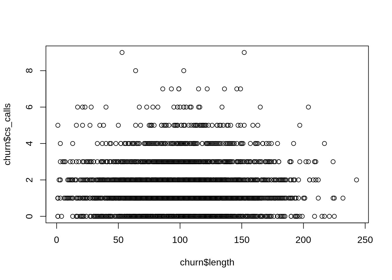
This plot can be helpful, but it isn’t production quality. Typically when we want to make nice-looking plots we use the ggplot2 package (Wickham et al. 2018):
library(ggplot2)
ggplot(churn,aes(x=length,y=cs_calls)) + geom_point() +
   scale_x_continuous(name="Account length") +
   scale_y_continuous(name="Customer service calls")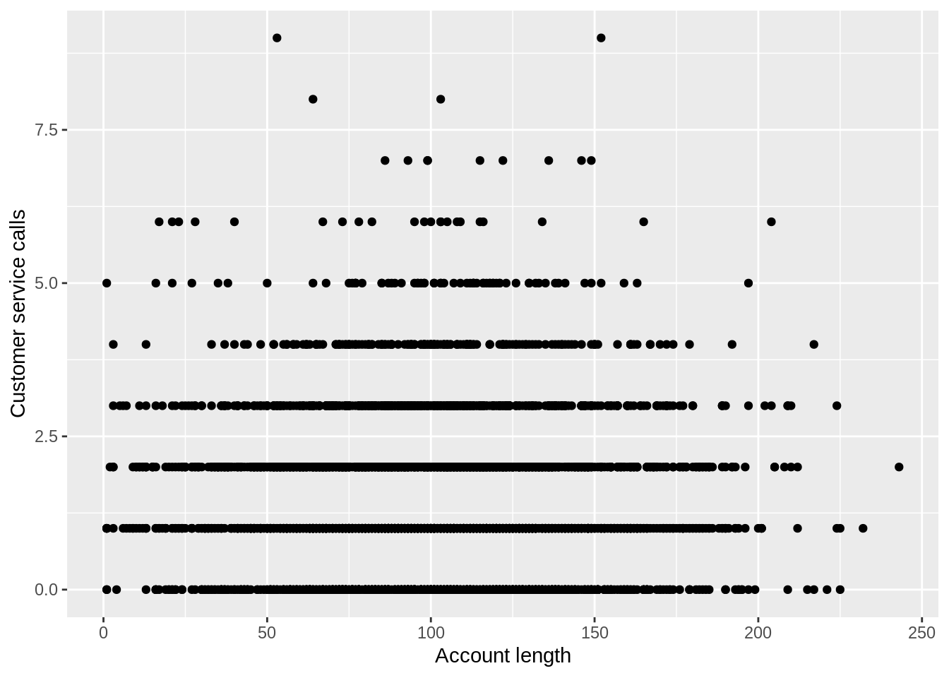
The code here looks complicated, but if we break it down, it becomes clear. The ggplot command sets up our axes. This specifies that our data is churn and the x and y variables are going to be length and cs_calls. Then we added points to this plot with the geom_point() command. The other commands are just setting the axis labels and are not necessary. You can find a ggplot command for almost every kind of static plot you can think of. This reference has 50 different ggplots that you can use to create almost any kind of visualization you could want.
2.1.2.4 Merging data
2.1.2.5 Structure of databases
2.1.2.6 Connecting to databases
To connect to sql databases (specifically the wooldridge2 database we are going to use almost exclusively), we are going to use the DBI package (R Special Interest Group on Databases (R-SIG-DB), Wickham, and Müller 2018) and RSQLite package (Müller et al. 2018). Install those packages and then you can call:
library(DBI)This command loads the DBI library which has the procedures for working with databases. Then we are then going to use the RSQLite library to access the wooldridge2.db.
con <- dbConnect(RSQLite::SQLite(),'wooldridge2.db')dbConnect from DBI opens a connection to the database. The file is now “in use” and cannot be modified by other programs until we close the connection. To see what is in the database (the table names) we can call:
dbListTables(con)## [1] "401k" "401k_labels" "401ksubs"
## [4] "401ksubs_labels" "admnrev" "admnrev_labels"
## [7] "affairs" "affairs_labels" "airfare"
## [10] "airfare_labels" "alcohol" "alcohol_labels"
## [13] "apple" "apple_labels" "athlet1"
## [16] "athlet1_labels" "athlet2" "athlet2_labels"
## [19] "attend" "attend_labels" "audit"
## [22] "audit_labels" "barium" "barium_labels"
## [25] "beauty" "beauty_labels" "benefits"
## [28] "benefits_labels" "beveridge" "beveridge_labels"
## [31] "big9salary" "big9salary_labels" "bwght"
## [34] "bwght2" "bwght2_labels" "bwght_labels"
## [37] "campus" "campus_labels" "card"
## [40] "card_labels" "cement" "cement_labels"
## [43] "ceosal1" "ceosal1_labels" "ceosal2"
## [46] "ceosal2_labels" "charity" "charity_labels"
## [49] "consump" "consump_labels"Now if we want to pull a particular table from the database, we can use the dbReadTable function on the connection with the table name. This function returns a data.frame object. Because we prefer data.tables, we are then going to migrate the data.frame to a data.table with the data.table() function and store that data.table as a variable:
bwght <- data.table(dbReadTable(con,'bwght'))In the wooldridge2 database, every table of data has some labels describing that data. To see the labels for the bwght data, call:
dbReadTable(con,'bwght_labels')## index variable.name type format variable.label
## 1 0 faminc float %9.0g 1988 family income, $1000s
## 2 1 cigtax float %9.0g cig. tax in home state, 1988
## 3 2 cigprice float %9.0g cig. price in home state, 1988
## 4 3 bwght int %8.0g birth weight, ounces
## 5 4 fatheduc byte %8.0g father's yrs of educ
## 6 5 motheduc byte %8.0g mother's yrs of educ
## 7 6 parity byte %8.0g birth order of child
## 8 7 male byte %8.0g =1 if male child
## 9 8 white byte %8.0g =1 if white
## 10 9 cigs byte %8.0g cigs smked per day while pregNow all there is left to do is disconnect from the database:
dbDisconnect(con)This closes the connection so that other programs can use or manipulate the file again. Don’t memorize these database commands. Below, we will write a wrapper function for all these operations so that we don’t have to remember them specifically.
2.1.3 Control structures
2.1.3.1 If statements
If statements are one of the core building blocks of computer code. If a condition is met, we are going to execute some code. Before we do this, let’s create a number x:
x <- rnorm(1,mean=5,sd=1)
x
## [1] 4.556368Here x was randomly created, so I (the author) don’t know whether it is less than \(5\) or greater than \(5\) because the code hasn’t been executed at the time I’m writing this. Now look at the following if statement:
if(x < 5){
  print("x less than 5")
}
The code here (if it were executed) would first check if the statement in the parentheses is true (i.e., x<5). If it is true, it will execute the code in the brackets (i.e., print("x less than 5")). So if x is less than \(5\), this would print out “x less than 5”. We can also add a case for when the condition is false using the else clause:
if(x < 5){
  print("x less than 5")
}else{
  print("x greater than 5")
}
## [1] "x less than 5"Here you can see the output which will either say “x less than 5” or “x greater than 5”.
2.1.3.2 For loops
The second basic building block of coding is looping. For this purpose, we are going to use the for loop. A for loop is a loop that runs for a specific number of cycles. It uses an iterator which is a variable that grows or shrinks each cycle. The following loop uses the iterator i which starts at \(1\) and grows to \(5\) by steps of \(1\). So i goes \(1\), \(2\), \(3\), \(4\), and then \(5\) and the loop is over. The code inside the brackets is going to be run each time. So for each value of i, R is going to print that value. So this loop prints the numbers \(1\) to \(5\), one at a time:
for(i in 1:5){
  print(i)
}
## [1] 1
## [1] 2
## [1] 3
## [1] 4
## [1] 5We can loop over other sets too. For instance the seq(a,b,c) function can be used to grow a number from a to b by units of c:
for(i in seq(0,1,0.2)){
  print(i)
}
## [1] 0
## [1] 0.2
## [1] 0.4
## [1] 0.6
## [1] 0.8
## [1] 12.1.3.3 User-defined functions
The last import building block of computer code is the user-defined function. Here I am going to create a sample standard deviation function. This function already exists in R, so this is an illustration of the concept of creating functions rather than a practical example of a code which is going to save us time. Below in section 2.4.1.5, we are going to create a function that is actually helpful to us. To define a function, you just have to save the function call to a variable name (e.g., sd):
sd <- function(data){
  val <- var(data)
  val <- sqrt(val)
  return(val)
}
Here we are defining the sd function. This function takes some input data. At the end of the function, the function is going to output something using the return call. Here we are returning val. So how is R going to calculate val? First val is obtained by finding the sample variance of data. Once we have the sample variance, we are going to modify val by taking its square root: val <- sqrt(val). Then we simply return val to the user. So:
sd(rnorm(100,mean=5,sd=2))## [1] 2.233749is about \(2\).
2.1.3.4 wpull function
References
Dowle, Matt, and Arun Srinivasan. 2019. Data.table: Extension of ‘Data.frame‘. https://CRAN.R-project.org/package=data.table.
Wickham, Hadley, Winston Chang, Lionel Henry, Thomas Lin Pedersen, Kohske Takahashi, Claus Wilke, and Kara Woo. 2018. Ggplot2: Create Elegant Data Visualisations Using the Grammar of Graphics. https://CRAN.R-project.org/package=ggplot2.
R Special Interest Group on Databases (R-SIG-DB), Hadley Wickham, and Kirill Müller. 2018. DBI: R Database Interface. https://CRAN.R-project.org/package=DBI.
Müller, Kirill, Hadley Wickham, David A. James, and Seth Falcon. 2018. RSQLite: ’SQLite’ Interface for R. https://CRAN.R-project.org/package=RSQLite.