2.3 Probability
2.3.1 Random variables
2.3.1.1 Probability spaces
Before beginning any serious study of data science, it is critical to understand the basics of the random processes which created the data itself. This will allow us to understand the statistics we create as well as when those statistics are likely to fail.
Essentially we define a probability space as a collection of events \(\{E\}\) and their associated probabilities \(\text{Pr}[E]\).
A random variable \(X\) is a function which outputs different number values based on the events that happen in the probability space. For instance, when a dice is rolled, whichever side faces up is labeled with a number \(1\) to \(6\). Thus \(X\) could be that number and the sample space, \(\Omega\), would be the integer numbers \(1, 2, 3, 4, 5,\) and \(6\). The sample space could be a set of discrete numbers (like \(1\) to \(6\)) or it could be a continuous set like the real numbers \((-\infty,\infty)\) for something like a normal random variable.
2.3.1.2 Density functions
When it comes to random variables, we have four main categories: discrete, continuous, mixed, and singular. Discrete random variable have probability mass functions. Continuous random variables have probability density functions. Mixed random variables are combinations of discrete and continuous random variables and will be discussed in ??. We will not be concerned with singular random variables as they are mathematical curiosities, but not directly applicable for data science at the time of writing.
The probability density function (PDF) is a function which describes where the concentration of probability for the random variable lies: \[\text{Pr}[a < X\leq b] = \int_a^bf(x)dx\] Hence, the function must integrate to one \(\int_{-\infty}^\infty f(x)dx=1\) so that the total probability is one. The cumulative distribution function (CDF) is the integral of the PDF: \[F(t)=\int_{-\infty}^t f(x)dx=\text{Pr}[X\leq t]\]
For discrete random variables, there is no probability density function. Instead, we have a probability mass function (PMF) which behaves similarly: \[\text{Pr}[a\leq x\leq b] = \sum_{i=a}^b f(x)\] Just like the PDF must integrate to one, the PMF must sum to one, i.e., \(\sum_{k\in \Omega}f(k)=1\). The CDF for a discrete random variable is: \[F(t)=\sum_{x\leq t} f(x)dx=\text{Pr}[X\leq t]\]
As we have mentioned, a distribution may or may not have a PDF or a PMF. That said, all random variables must have a CDF. The CDF is guaranteed, but the PDF or PMF is optional.
2.3.1.3 Distribution moments
The first two moments of a distribution are its mean and variance. The mean or expected value of any continuous variable is \[\text{E}[X]=\int_{-\infty}^\infty x\;f(x)\;dx\] The expected value or mean is a measure of the center of the distribution. It is an average of the random variable weighted by the probability density function. If the variable is discrete, then \(\text{E}[X]=\sum_{x\in\Omega} x\;f(x)\). The expected value of any function of a random variable is:
\[\text{E}[g(X)]=\int_{-\infty}^\infty g(x)\;f(x)\;dx\] This means that any linear function of a random variable can be found as
\[\text{E}[aX+b]=\int_{-\infty}^\infty (a X + b)\;f(x)\;dx=a\text{E}[X]+b\]
If we have two random variables (we will discuss joint probability later), then
\[\text{E}[X+Y]=\text{E}[X]+\text{E}[Y]\]
The variance of a random variable represents the spread of that variable. A higher variance means a larger spread. Variance is defined as \[\text{Var}[X]=\text{E}[(X-\text{E}[X])^2]=\text{E}[X^2]-\text{E}[X]^2\] Take special note that while expected value can be applied across linear functions, that doesn’t mean that it can be applied to quadratics or other non-linear functions. Otherwise the variance would always be zero because \(\text{E}[X^2]\) would be equal to \(\text{E}[X]^2\).
The standard deviation is the square root of the variance:
\[\text{SD}[X]=\sqrt{\text{Var}[X]}\]
We often use standard deviation because it has the same units as the original data. The variance is related to the variable squared, so if the original data used meters then the variance would be in terms of square meters. This is awkward because square meters don’t make sense unless we are talking about area, and the problem could have nothing to do with area. So to put the variance in terms of the original data, we need to take the square root of the variance. In other words, we need to use the standard deviation to better interpret our results.
It is possible for the moments of distribution to not exist. For instance, if the integral of \(x^2\;f(x)\;dx\) evaluated from \(-\infty\) to \(\infty\) diverges to \(\infty\), then the distribution is said to not have a variance. Such a variable would have such a serious variance that it does not even exist. This kind of variable is extremely uncertain and is one way to model risky phenomena. Most random variables have some mean and some variance and for the most part, we are going to assume that our variables have these defined. When this assumption is not true we are going to have to change our approach.
2.3.1.4 Higher moments
2.3.1.5 Common distributions
2.3.1.5.1 Uniform distribution
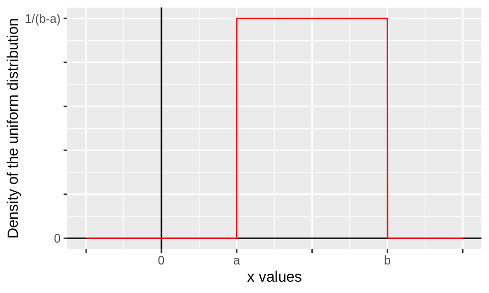
The two most important distributions we are going to use for this class are the uniform distribution and the normal distribution. The uniform distribution is where the probability is evenly distributed in the range of the output. To indicate that a variable has a uniform distribution we write: $ X U[a,b] $. This indicates that \(X\) has a uniform \([a,b]\) distribution. This distribution has two “parameters,” \(a\) and \(b\). Distributions will have any number of parameters. \(a\) here represents the lower bound of the distribution. \(b\) represents the upper bound of the distribution. So the range is from \(a\) to \(b\). The PDF for this distribution is: \[ f(x) = \begin{cases} \frac{1}{b-a},& \text{if } x\in [a,b]\\ 0, & \text{otherwise} \end{cases} \]
The PDF is defined to be zero outside of the interval where our variable is going to fall \([a,b]\). In the interval \([a,b]\), the variable is defined to be flat or a constant value. The following figure is a plot of the uniform distribution’s PDF:
The expected value of the uniform distribution is \[\text{E}[Y]=\int_a^b y\;f(y)\;dy=\int_a^b \frac{y}{b-a}dy=\frac{1}{2}\frac{b^2-a^2}{b-a}\]
or \(\text{E}[Y]=\frac{a+b}{2}\). This is intuitive because the mean value should be right in the center of the distribution or directly between \(a\) and \(b\). The variance of \(Y\) can be calculated similarly and is \(\text{Var}[Y]=\frac{(b-a)^2}{12}\).
2.3.1.5.2 Normal distribution
The normal distribution is another continuous distribution which is hugely important for our work. We denote that a variable \(Y\) is normally distributed by \(Y \sim \mathcal{N}(\mu,\sigma^2)\). The PDF for the normal distribution is: \[f(x) = \frac{1}{\sqrt{2\pi\sigma^2}}\exp \begin{bmatrix} -\frac{(x-\mu)^2}{2\sigma^2}\end{bmatrix}\] The PDF of the normal distribution has the following shape: 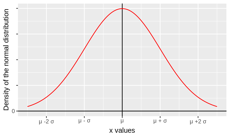
The normal distribution has two parameters, \(\mu\) and \(\sigma^2\). The normal distribution is symmetric around \(mu\) so all the common measures of centrality agree that \(\mu\) is at the center of distribution. Hence, we can show that \[\text{E}[Y]=\int_{-\infty}^{\infty} y\;f(y)\;dy=\mu\]. The derivation of this is omitted from this book not because it is difficult calculus (it isn’t) but because we are going to use this value often as a reference. We know what the mean of normal numbers is. We don’t need to calculate it to be able to use it.
The \(\sigma^2\) parameter represents the spread of the distribution. When \(\sigma^2\) is large, the distribution has a wider shape. When \(\sigma^2\) is smaller, the distribution is more concentrated around \(\mu\). The variance of the normal distribution \(\sigma^2\), i.e., \(\text{Var}[Y]=\sigma^2\). Thus we can say that the normal distribution is parameter by its mean and variance which is to say that if we know those two numbers, we know the particular distribution uniquely.
A special case of the normal distribution is the standard normal distribution which is defined where \(\mu=0\) and \(\sigma^2=1\). This specific normal distribution is “standardized” meaning that it has mean zero and variance one.
2.3.1.5.3 Log-normal distribution
\[\ln Y \sim \mathcal{N}(\mu,\sigma^2)\] \[f(x) = \frac{1}{x\sqrt{2\pi\sigma^2}}\exp{\Big( -\frac{(\ln x-\mu)^2}{2\sigma^2}\Big)}\] \[\text{E}[Y]=\exp\begin{pmatrix}\mu+\frac{\sigma^2}{2}\end{pmatrix}\] \[\text{Var}[Y]=\big[\exp(\sigma^2)-1\big]\exp\big(2\mu+\sigma^2\big)\]
2.3.1.5.4 Binomial distribution
\[Y \sim \mathcal{B}(n,p)\] \[f(k) = \begin{pmatrix}n\\k\end{pmatrix} p^k(1-p)^{n-k} \; \text{for} \; k=0,1,\dots,n\] \[\text{E}[Y]=np\] \[\text{Var}[Y]=np(1-p)\]
2.3.1.5.5 Poisson distribution
\[Y\sim \text{Poisson}(\lambda)\] \[f(k)=\frac{\lambda^k e^{-\lambda}}{k!} \; \text{for} \; k=0,1,\dots\] \[\text{E}[Y]=\lambda\] \[\text{Var}[Y]=\lambda\]
2.3.1.5.6 Gamma distribution
\[Y\sim \text{Gamma}(\alpha,\beta)\] \[f(x)=\frac{\beta^\alpha x^{\alpha-1} e^{-\beta x}}{\Gamma(\alpha)} \; \text{for} \; x\in[0,\infty)\] \[\text{E}[Y]=\frac{\alpha}{\beta}\] \[\text{Var}[Y]=\frac{\alpha}{\beta^2}\]
2.3.1.5.7 Exponential distribution
\[Y\sim \text{Exponenial}(\lambda)\] \[f(x)=\lambda e^{-\lambda x} \; \text{for} \; x\in[0,\infty)\] \[\text{E}[Y]=\frac{1}{\lambda}\] \[\text{Var}[Y]=\frac{1}{\lambda^2}\]
2.3.1.5.8 Student t-distribution
\[Y\sim t_r\] \[f(x)=\frac{\Gamma(\frac{r+1}{2})}{\sqrt{r\pi}\Gamma(\frac{r}{2})}\begin{pmatrix}1+\frac{x^2}{r}\end{pmatrix}^{-\frac{r+1}{2}}\] \[\text{E}[Y]=0 \;\text{if}\; r>1\] \[\text{Var}[Y]=r/(r-2) \;\text{if}\; r>2\]
2.3.1.5.9 Chi-squared distribution
\[Y\sim \chi^2_r\] \[Y=\sum_{i=1}^r X_i^2 \; \text{where}\; X_i\sim \mathcal{N}(0,1)\] \[f(x)=\begin{cases} \frac{x^{r/2-1}\exp(-x/2)}{2^{r/2}\Gamma(r/2)},& \text{if } x>0\\ 0, & \text{otherwise} \end{cases}\] \[\text{E}[Y]=r\] \[\text{Var}[Y]=2r\]
2.3.1.5.10 Bernoulli random walk distribution
\[Y_t=\sum_{i=0}^t X_i\;\text{where}\; X_i\sim 2\mathcal{B}(1,0.5)-1\]
\[f(k)=\begin{cases} \frac{1}{2^t}\begin{pmatrix}t\\ \frac{t+k}{2}\end{pmatrix},& \text{if } t+k \,\text{is even and}\, |t|\leq n\\ 0, & \text{otherwise} \end{cases}\]
\[\text{E}[Y_t]=0\] \[\text{Var}[Y_t]=\sum_{i=0}^t Var[X_i] = t\]
2.3.1.6 Sample statistics
When we have a sample of data, we are going to think of the data a multiple observations of the same variable. For instance we might have a sample \(x_1,\dots,x_n\) which would index \(x_i\) where \(i=1,\dots,n\). From this sample, we can calculate the sample mean. The sample is different from the mean of random variables we described above. That was a population mean or what we would expect from the random variable if we knew the distribution already. The sample mean can be found by averaging the points that we observe or:
\[\overline{x}=n^{-1}\sum\nolimits_{i=1}^n x_i\]
In the statistics section, we will discuss the distribution of the sample mean. Similar to the sample mean, we can calculate the sample variance which we will call \(s^2\):
\[s^2=(n-1)^{-1}\sum\nolimits_{i=1}^n (x_i-\overline{x})^2\]
Taking the square root of \(s^2\) gives us \(s\) which is the sample standard deviation.
2.3.1.7 Order statistics
2.3.2 Joint distributions
When we have more than one variable in our data, the interaction between these variables can be modeled with joint probability. This is a complex subject, but the results can be very interesting. For two continuous variables, there is a joint probability density function or joint PDF: \(f(x,y)\). This is a function of two variables. It takes two inputs \(x\) and \(y\) and outputs one probability density such that: \[\int_{\Omega x}\int_{\Omega y}f(x,y)\;dy\;dx=1\]
We can visualize a joint distribution as follows:
In general, we can have up to \(r\) variables in a joint distribution, \(f(x_1,\dots,x_r)\). Obviously this is more complicated and cannot be visualized in a three dimensional world.2.3.2.1 Marginal distributions
Every joint distribution is going to have marginals. Marginals are basically the individual PDF for each of the variables in a joint density. So if we have two variables, \(x\) and \(y\) then we are going to have two marginal distributions-one for \(x\) and one for \(y\): \[f_x(x)=\int_{\Omega y}f(x,y)\;dy\] \[f_y(y)=\int_{\Omega x}f(x,y)\;dx\]
As you can see here, we get back to the marginal by integrating across the other variables. This means that we are ignoring the other variables when we think about the marginal density of \(y\).
2.3.2.2 Conditional distributions
If we knew the value of \(x\), then we could use that information to predict \(y\). This is the principle behind conditional distributions. In the world where \(x\) is known, where should we expect \(y\) in probability? That means that conditional probability is a function of a known \(x\) value. We define conditional probability of \(y\) on \(x\) as follows:
\[f_{y|x}(y|x)=\frac{f(x,y)}{f_x(x)}\]
Notice that this conditional probability must integrate to one: \[\int_{\Omega x} f_{x|y}(x|y)\;dx=1\]
We can also turn this around and find the conditional probability of \(x\) on \(y\): \[f_{x|y}(x|y)=\frac{f(x,y)}{f_y(y)}\]
This leads us into Bayes’ theorem.
2.3.2.3 Bayes’ theorem
Bayes theorem is fundamentally a consequence of the definition of conditional distributions. We know that \(f_{x|y}(x|y)f_y(y)=f(x,y)\) and we know \(f_{y|x}(y|x)f_x(x)=f(x,y)\). Therefore, we can write \(f_{x|y}(x|y)f_y(y)=f_{y|x}(y|x)f_x(x)\) or
One primary application of this idea is for understanding the probability of having a disease given a positive test: \[\text{Pr}[\text{disease|test positive}]=\frac{\text{Pr}[\text{positive test|disease}]\text{Pr}[\text{disease}]}{\text{Pr}[\text{positive test}]}\] or in other words, the probability of having the disease given that you tested positive is the probability of testing positive given that you have the disease times the probability of having the disease in general over the probability of having a positive test. This allows use to update the probability that you have the disease if we know that you have a positive test result. This is called Bayesian updating.
Consider the following example: Let’s suppose that the probability of testing positive if you have the disease is 1. Also suppose that the false positive rate is \(1/100\). Let’s also suppose that the prevalence of the disease in the overall population is \(1/1000\). Now today you take the test and get a positive result. Importantly, I’m assuming that there’s absolutely no other reason to assume that you have this disease. If there were some other symptom, then you shouldn’t be compared to the average person in the population, but rather to other people with the symptom and that would change the situation entirely. Now the probability of having the disease is \(1/1000\). The probability of testing positive for the disease given that you have the disease is 1. But the probability of a positive test overall is \(\text{Pr}[\text{positive test}]=\text{Pr}[\text{positive test|disease}]\text{Pr}[\text{disease}]+\text{Pr}[\text{positive test|no disease}]\text{Pr}[\text{no disease}]=1*1/1000+1/100*999/1000=0.011\). Therefore, the probability that you have the disease is \(\text{Pr}[\text{disease|positive test}]=0.091\) or a little less than \(10\%\). Even though you tested positive the false negative rate is \(0\) and the false positive rate is \(1/100\), you’re probably fine. This example is why good doctors won’t test you for diseases without some other indication that you have the illness.
2.3.2.4 Covariance and correlation
The covariance is defined to be similar to the variance. Essentially we are looking at the connection between two random variable. When \(X\) has a large deviation from its mean, what is the average deviation in \(Y\)?We can calculate the sample covariance and sample correlation as follows: \[s_{x,y}=(n-1)^{-1}\sum\nolimits_{i=1}^n (x_i-\overline x)(y_i-\overline y)\] \[r_{x,y}=\frac{s_{x,y}}{s_x s_y}\]
To calculate the sample covariance and sample correlation in R, we can use cov() and cor() functions:
cov(churn$length,churn$cs_calls) # Sample covariance## [1] -0.1988526cor(churn$length,churn$cs_calls) # Sample correlation## [1] -0.0037959392.3.2.5 Independence
Independence is an extremely important concept with a particularly terrible (intuitively) definition:
This condition is extremely powerful when true. When it is, then any expected value between the two variables can be calculated by taking the expected value of the \(X\) part and the \(Y\) part separately. or \(\text E[f(X)g(Y)]=\text E[f(X)]\text E[g(Y)]\). This implies among other things that: \[\text{Cov}[X,Y]=\text E[(X- \text E[X])(Y-\text E[Y])]=(\text E[X-\text E[X]])(\text E[Y-\text E[Y]])=0\] This means that whenever we have independent variables, they must be uncorrelated. In other words, if we see a correlation, that implies some kind of dependence. We will discuss circumstances later where this is not true, but in the classic statistical framework, this is the implication. Independence is an extremely powerful assumption with many un-intuitive consequences. We will be discussing these consequences in this course. When independence is not present, our standard models can result in interesting failures. We will be discussing those failures as well.
2.3.2.6 Independent identically distributed
When we are working on data, our standard model is going to be that the data is independent and identically distributed or (iid) with some mean (\(\mu\)) and some variance (\(\sigma^2\)) or \[x_i \sim iid(\mu,\sigma^2) \;\text{for}\;i=1,\dots,n\]
What this assumption says is that each row of our data should be completely unrelated to its neighbors and that every row represents a draw from the same distribution. This means that if the marginal PDF of \(x_1\) is \(f(x_1)\), then the joint PDF can be written: \[f(x_1,\dots,x_n)=\prod_{i=1}^n f(x_i).\]
This is very convenient mathematically. Also note that the assumption implies that the distribution from which the data is drawn has some finite mean and variance, even if we have no idea what the mean, variance, and distribution of the data are.
2.3.2.7 Matrix moments
\[\mathbf{A} = \begin{bmatrix}a_{ij}\end{bmatrix}\] \[\text{E}[\mathbf{A}] = \begin{bmatrix}\text{E}[a_{ij}]\end{bmatrix}\] \[\text{Var}[x]=\text{E}[(x-\mu)(x-\mu)'] \;\text{where}\; \mu=\text{E}[x]\]
2.3.2.8 Multivariate normal distribution
The distribution featured above was a multivariate normal distribution. If you know matrix algebra, then we can express the multivariate normal distribution as follows: \[x \sim \mathcal{N}_r(\mu,\Sigma)\]
Here \(x\) and \(\mu\) are \(r\times1\) vectors and \(\Sigma\) is an \(r\times r\) matrix. Using these numbers, we can define the multivariate normal PDF as follows: \[f(x)=(2\pi)^{-k/2}|\Sigma|^{-1/2}\exp\begin{bmatrix}-\frac{1}{2}(x-\mu)'\Sigma^{-1}(x-\mu)\end{bmatrix}.\]
Once we have covered covariance and matrix moments, we can explain the intuition behind the \(\mu\) and \(\Sigma\) parameters. Effectively, \(\mu\) is the mean of the distribution, and \(\Sigma\) is the variance-covariance matrix of the \(x\) variables.
2.3.2.9 Conditional normal distribution
\[x_1|x_2\sim \mathcal{N}_{r_1}(\overline\mu,\overline\Sigma)\] \[\overline\mu=\mu_1+\Sigma_{12}\Sigma_{22}^{-1}(x_2-\mu_2)\] \[\overline\Sigma=\Sigma_{11}-\Sigma{12}\Sigma_{22}^{-1}\Sigma_{21}\]
2.3.2.10 Cumulants
2.3.3 Group-by
Most questions people typically have about data can be answered with summary statistics alone. Suppose we want to know how our sales change seasonally. To answer the question, we just have to group our sales by the month (or even quarter) and add up the sales numbers. Do this for the last 3 years and with 12 numbers, we can easily see how things change month-to-month. This information could be displayed in a basic figure or even in a simple table. Aggregating data like this is known as a “group by” statement following notation from SQL. Effectively we are grouping by the month and then calculating a sum or mean of the variables in question. Being able to think and write clever group by statements to answer data questions is an art that gets better with practice.
2.3.3.1 Referencing data.tables
The general notation for a data.table is dt[row,column,by=group] so if we want to call the first row:
churn[1,]## length intl_plan vm_plan cs_calls churn bill mins calls
## 1: 128 0 1 1 0 75.56 717.2 303And if we want the first column:
churn[,1]## length
## 1: 128
## 2: 107
## 3: 137
## 4: 84
## 5: 75
## ---
## 3329: 192
## 3330: 68
## 3331: 28
## 3332: 184
## 3333: 74And if we want the first element overall:
churn[1,1]## length
## 1: 128In the row area, we can subset the data set where a particular condition is true. So if we wanted only the people who called customer service more than 7 times, we would type churn[cs_calls>7,] which produces:
##    length intl_plan vm_plan cs_calls churn  bill  mins calls
## 1:    152         1       1        9     1 77.68 770.3   297
## 2:     64         0       1        8     0 64.67 617.4   303
## 3:    103         0       0        8     1 52.73 551.3   363
## 4:     53         0       0        9     1 63.10 598.7   366
If we want to then find the mean of churn for the people with more than 7 customer service calls:
churn[cs_calls>7,mean(churn)]## [1] 0.75To group by a particular variable we use two commas in the call with by= set to the variable we wish to group by. Here, I am going to group by customer service calls and find the mean of churn for people who called customer service 0 times, 1 time, 2 times, etc:
churn[,mean(churn),by=cs_calls]## cs_calls V1
## 1: 1 0.1033023
## 2: 0 0.1319943
## 3: 2 0.1146245
## 4: 3 0.1025641
## 5: 4 0.4578313
## 6: 5 0.6060606
## 7: 7 0.5555556
## 8: 9 1.0000000
## 9: 6 0.6363636
## 10: 8 0.5000000To find out how many people are in each group, we can use the .N variable:
churn[,.N,by=cs_calls]## cs_calls N
## 1: 1 1181
## 2: 0 697
## 3: 2 759
## 4: 3 429
## 5: 4 166
## 6: 5 66
## 7: 7 9
## 8: 9 2
## 9: 6 22
## 10: 8 2Often it is helpful to use find two variables for each group. the .() function can be used to combine multiple variables in a data.table:
churn[,.(.N,mean(churn)),by=cs_calls] ## cs_calls N V2
## 1: 1 1181 0.1033023
## 2: 0 697 0.1319943
## 3: 2 759 0.1146245
## 4: 3 429 0.1025641
## 5: 4 166 0.4578313
## 6: 5 66 0.6060606
## 7: 7 9 0.5555556
## 8: 9 2 1.0000000
## 9: 6 22 0.6363636
## 10: 8 2 0.5000000Because the numbers that come out are not ordered, we might want to impose an order on the rows by sorting:
churn[order(cs_calls),.(.N,mean(churn)),by=cs_calls]## cs_calls N V2
## 1: 0 697 0.1319943
## 2: 1 1181 0.1033023
## 3: 2 759 0.1146245
## 4: 3 429 0.1025641
## 5: 4 166 0.4578313
## 6: 5 66 0.6060606
## 7: 6 22 0.6363636
## 8: 7 9 0.5555556
## 9: 8 2 0.5000000
## 10: 9 2 1.0000000It is unfortunate that many data.table operations remove the column names. To fix this we can save our result as a new variable and then rename the columns:
outp <- churn[order(cs_calls),.(.N,mean(length),mean(bill),mean(churn)),by=cs_calls]
names(outp) <- c('cs_calls','N','length','bill','churn')
outp
## cs_calls N length bill churn
## 1: 0 697 101.30273 59.90430 0.1319943
## 2: 1 1181 101.77985 59.46177 0.1033023
## 3: 2 759 99.22530 58.89424 0.1146245
## 4: 3 429 101.43357 59.83657 0.1025641
## 5: 4 166 102.66265 60.22337 0.4578313
## 6: 5 66 102.56061 58.14697 0.6060606
## 7: 6 22 90.18182 54.23636 0.6363636
## 8: 7 9 116.11111 56.84444 0.5555556
## 9: 8 2 83.50000 58.70000 0.5000000
## 10: 9 2 102.50000 70.39000 1.0000000Because this process is tedious and we often just want the mean of the variables, we can use the lapply function applied to each column (.SD for subset data).
churn[,lapply(.SD,mean),by=cs_calls]| cs_calls | length | intl_plan | vm_plan | churn | bill | mins | calls |
|---|---|---|---|---|---|---|---|
| 1 | 101.77985 | 0.0948349 | 0.2912786 | 0.1033023 | 59.46177 | 592.1865 | 306.2159 |
| 0 | 101.30273 | 0.1190818 | 0.2769010 | 0.1319943 | 59.90430 | 595.4574 | 304.9484 |
| 2 | 99.22530 | 0.0816864 | 0.2832675 | 0.1146245 | 58.89424 | 588.2964 | 305.5599 |
| 3 | 101.43357 | 0.0885781 | 0.2284382 | 0.1025641 | 59.83657 | 593.7618 | 302.2331 |
| 4 | 102.66265 | 0.1265060 | 0.2530120 | 0.4578313 | 60.22337 | 595.6663 | 305.3434 |
| 5 | 102.56061 | 0.0909091 | 0.2575758 | 0.6060606 | 58.14697 | 575.9788 | 303.1364 |
| 7 | 116.11111 | 0.0000000 | 0.2222222 | 0.5555556 | 56.84444 | 586.5111 | 310.8889 |
| 9 | 102.50000 | 0.5000000 | 0.5000000 | 1.0000000 | 70.39000 | 684.5000 | 331.5000 |
| 6 | 90.18182 | 0.0000000 | 0.4090909 | 0.6363636 | 54.23636 | 560.3182 | 292.4091 |
| 8 | 83.50000 | 0.0000000 | 0.5000000 | 0.5000000 | 58.70000 | 584.3500 | 333.0000 |
This is a fairly advanced function, so don’t be discouraged if this seems fairly complicated. We will discuss lapply functions later. For now you just need to know that they can be used to calculate the mean across many variables in a data.table. We can also apply the variance (var) or standard deviation (sd) function instead:
churn[,lapply(.SD,sd),by=cs_calls]| cs_calls | length | intl_plan | vm_plan | churn | bill | mins | calls |
|---|---|---|---|---|---|---|---|
| 1 | 39.95407 | 0.2931109 | 0.4545441 | 0.3044822 | 10.474178 | 90.39080 | 34.73712 |
| 0 | 39.51951 | 0.3241173 | 0.4477885 | 0.3387276 | 10.870004 | 94.17884 | 34.87746 |
| 2 | 41.26656 | 0.2740670 | 0.4508823 | 0.3187783 | 10.178406 | 86.36005 | 33.80545 |
| 3 | 39.56490 | 0.2844655 | 0.4203166 | 0.3037429 | 10.311986 | 88.24242 | 34.19470 |
| 4 | 35.08130 | 0.3334246 | 0.4360532 | 0.4997261 | 10.896284 | 90.46204 | 35.15329 |
| 5 | 36.14081 | 0.2896827 | 0.4406501 | 0.4923660 | 11.463548 | 93.87850 | 34.24702 |
| 7 | 23.53956 | 0.0000000 | 0.4409586 | 0.5270463 | 8.525984 | 86.41013 | 29.71298 |
| 9 | 70.00357 | 0.7071068 | 0.7071068 | 0.0000000 | 10.309617 | 121.33952 | 48.79037 |
| 6 | 46.41596 | 0.0000000 | 0.5032363 | 0.4923660 | 7.964978 | 62.79750 | 25.06118 |
| 8 | 27.57716 | 0.0000000 | 0.7071068 | 0.7071068 | 8.442855 | 46.73976 | 42.42641 |
Here we are seeing the standard deviation of each variable for each of the groups based on number of customer service calls.
2.3.3.2 Group-bys with continuous variables
Sometimes we want to perform group-by statements, but our data is continuous. When we group by a continuous variable, we get the following result:
churn[order(length),.(.N,mean(churn)),by=length]## length N V2
## 1: 1 8 0.125
## 2: 2 1 1.000
## 3: 3 5 0.000
## 4: 4 1 0.000
## 5: 5 1 0.000
## ---
## 208: 221 1 0.000
## 209: 224 2 0.500
## 210: 225 2 0.500
## 211: 232 1 0.000
## 212: 243 1 0.000You can see here that length takes too many values and so the outcome isn’t clear. One possible solution to this is just to reverse the process:
churn[order(churn),.(.N,mean(length)),by=churn]## churn N V2
## 1: 0 2850 100.7937
## 2: 1 483 102.6646While this works here, it will not work in cases where our target variable (e.g., churn$churn) is continuous also. To deal with this we are going to “bin” the length variable. First we need to define the bin. Consider the following sequence command:
seq(0,250,25)## [1] 0 25 50 75 100 125 150 175 200 225 250This is going to be used to define the bins. We are going to cut() the length variable using these bins (include.lowest is just a parameter which specifies whether the lowest bin should include zero):
churn$length_bins <- cut(churn$length,seq(0,250,25),include.lowest=TRUE)
table(churn$length_bins)
##
## [0,25] (25,50] (50,75] (75,100] (100,125] (125,150] (150,175]
## 99 242 548 775 787 526 239
## (175,200] (200,225] (225,250]
## 91 24 2Now you can see that our data has been put into the bins we wanted. Now we can group by:
churn[order(length_bins),lapply(.SD,mean),by=length_bins]<!--
| length_bins | length | intl_plan | vm_plan | cs_calls | churn | bill | mins | calls |
|---|---|---|---|---|---|---|---|---|
| [0,25] | 14.77778 | 0.0808081 | 0.2727273 | 1.676768 | 0.1515152 | 59.97808 | 598.4828 | 297.0707 |
| (25,50] | 39.73967 | 0.0661157 | 0.2479339 | 1.487603 | 0.1198347 | 59.40798 | 587.9479 | 305.6157 |
| (50,75] | 64.45803 | 0.0930657 | 0.2846715 | 1.500000 | 0.1350365 | 59.64038 | 594.5024 | 304.7409 |
| (75,100] | 88.69806 | 0.0993548 | 0.2683871 | 1.596129 | 0.1496774 | 58.95072 | 589.8564 | 305.0697 |
| (100,125] | 112.85896 | 0.0889454 | 0.2858958 | 1.668361 | 0.1537484 | 59.49868 | 591.8094 | 304.1474 |
| (125,150] | 136.85741 | 0.1311787 | 0.3098859 | 1.484791 | 0.1406844 | 59.69844 | 593.4677 | 308.0304 |
| (150,175] | 161.17573 | 0.0920502 | 0.2217573 | 1.489540 | 0.1506276 | 60.33498 | 594.3397 | 306.9874 |
| (175,200] | 184.96703 | 0.0989011 | 0.2857143 | 1.395604 | 0.1318681 | 58.13451 | 580.3571 | 303.3297 |
| (200,225] | 211.25000 | 0.0416667 | 0.1666667 | 1.833333 | 0.2500000 | 59.47750 | 601.1167 | 303.6250 |
| (225,250] | 237.50000 | 0.0000000 | 0.0000000 | 1.500000 | 0.0000000 | 48.56500 | 510.8000 | 289.0000 |
--> |